
Valuing Rent Controlled Units: Are they as scary as some people think?
In the world of commercial real estate, one phrase can send inexperienced investors running for the hills: “Rent Control”. Negative headlines around rent control have been in the news frequently in recent years. The Biden administration vaguely proposed nationwide rent control, and major cities like NYC have enacted increasingly stricter rent control regulations. With all the negative press, we can understand why rent control is scary for investors. However, the question remains: is rent control as menacing as it is perceived? To understand this, we need to understand the different types of rent control, how they work, and how they impact the financials of a multifamily apartment complex.
When we started to dig into this topic, we were surprised to find a significant amount of publicly available information from acclaimed academics and economists on the macro effects of rent control, but very little assessing the micro impacts on individual properties. Having spotted this gap in knowledge, we decided to dig in and share our findings. Throughout the remainder of this Insight, we will present how we went about evaluating the impact of rent control on realized rents and provide data that will serve to simultaneously shine light on the fact that not all rent control regulations have a significant impact on project financials and assist others looking to assess rent controlled apartment complexes.
Before we can begin with the financials, we first need to understand the two primary types of rent control regulations.
Rent Control Units: This type of rent control is also commonly known as Vacancy Decontrol. Vacancy Decontrol means that when a tenant moves out, “Turnover,” the property manager can re-lease the apartment at market rate. However, when a tenant chooses to renew their lease, there is a set maximum by which the rent can be increased (typically tied to CPI).
Affordable Units: This type of rent control has a fixed maximum that a unit can be rented for. This maximum is typically set as a percentage of Area Median Income (AMI). The maximum does not reset to the market rate when a tenant moves out, however, Area Median Incomes are recalculated each year and tend to increase over time.
While Affordable Units are the stricter of the two types of rent control, they are easier to understand and project from a financial perspective. As such, they tend to be more approachable to inexperienced investors. At a high level, when assessing an Affordable Unit, you set rents at the current AMI restrictions (typically published by either the local municipality or the US HUD) and look at the historical change in AMI and assume that rents will increase by approximately that much moving forward. The financials are essentially the same as those for market rate units, but with a lower starting point and a different growth rate.
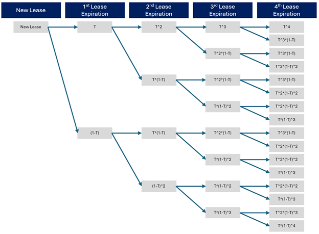
For Rent Controlled Units, the simple fact that rents are reset on turnover significantly increases the complexity of projecting realized rents. To understand why this is so complicated, let’s consider the trajectory of a single unit. Every time a lease expires, the tenant has the option to either vacate the unit, in which case rents are reset to the market rate, or to renew their lease, in which case rents are increased by the maximum rate set by regulation. This cycle continues until a tenant chooses to vacate the unit. As such, any given unit could be on its first lease (realized rents are at market rate), its first renewal (realized rents are at one period prior’s market rate and grown at the regulation-capped growth rate once), its second renewal (realized rents are at two period prior’s market rate grown at the regulation-capped growth rate twice), and so on, indefinitely. The tree of options (the first four renewal periods of which are shown below) grows exponentially.

It goes without saying that an exponentially growing number of trajectories is hard to project. For instance, if one is trying to model a 10-year hold period on a property, and they assume an average lease length of 12 months, in year 10, there are 1,024 possible trajectories that each apartment could have taken during that 10-year period. Luckily, it’s possible to dramatically reduce the complexity by looking at the probability of being in each state (Turnover, 1st Renewal, 2nd Renewal, etc.) rather than the path taken to get to each state. The chart below shows the probability of getting to each state.
For brevity, we will skip over the simplifying algebra, but if you do the math of simplifying the above figure, what you will find is that there are only three equations needed to describe the probability of being in any given state at any given time. For any given period “P” with an assumed annual turnover rate “T”, these are:
The probability of a unit having just turned over (Turnover) is T
The probability of a unit being on a given renewal is T*(1-P)^N, where “N” is the number of consecutive renewals ( 1st Renewal, 2nd Renewal, etc.)
The probability of a unit having never turned over is (1-T)^P

This realization dramatically simplifies the projections by allowing us to go from looking at the exponential number of trajectories to the linear number of states. As such, for the same 10-year period, we only need to look at 11 states.
By making simple assumptions about the turnover of rent-controlled units (T), we can now project what percentage of units will be in each state at any given time. The chart below shows what that looks like, assuming a 25% turnover (T = 0.25).

With a projection of state, we can then project the in-place rents for a given unit at any given time. Assuming a large enough sample size (a significant number of rent-controlled units), the law or large numbers should put these projections relatively close to what is experienced in real life.
Having worked through the math, we now want to look holistically across several scenarios to see if rent control regulations materially affected rents and present a significant risk to a property. To do so, we used our model to put together the following reference projections. The chart below shows the loss from rent control as a percentage of gross potential rent as a function of the difference between projected market rate rent growth, the rent control rent growth cap, and the assumed turnover rate. It’s worth noting that we have intentionally shown an unrealistically wide range of scenarios in order to allow readers to see a worst-case scenario and get a feel for the trends as a whole.

Looking at the above, the question remains whether investors should be wary of rent control. In our opinion, with some caveats discussed below, the above data says they should not. Let’s look through the individual factors to see how they affect loss.
Rent Growth Delta: The X-axis of the above chart shows how the difference between the rent growth cap and the market rate growth rate affects loss as a percentage of GPR. The scale of the X-axis can make this loss look staggering; however, given that most investors underwrite somewhere between 3% and 5% rent growth, this axis is misleading. This is because the maximum downside from Loss to Rent Control due to the Rent Growth factor is limited, with most of this axis representing a loss in upside potential. To illustrate this point, let’s look at an example. If an investor is looking to acquire a property, they believe that the local market will see 4% market rate rent growth, that rent control rent growth is tied to CPI, which they project at 2.5%, and that they will see 30% turnover of rent-controlled units. In this scenario, knowing the above, they would expect realized rents to be ~3.27% below market rate rents at steady state. This ~3.27% discount should be priced in at the time of acquisition. Now let’s consider the scenario where market rents increase by less than the projected 2.5% CPI Growth (Rent Control growth cap). Considering most rent control units will be below market from previous renewal caps, it is likely that rent can still be increased by the full projected 2.5% CPI cap. In this case, rent control serves to stabilize swings in market rent growth. If the full CPI cap can’t be realized, this is still the same market rate rent risk taken when investing in Non-Rent Controlled Units. Similarly, if market rate rents are above the 2.5% CPI projection, the business plan will improve as higher rents will be achieved when units turnover. The only scenario where rent-controlled units take additional risk is when the CPI comes in below 2.5% and the market rate rent growth is above it. It is unlikely that a significant gap exists here, given that housing costs are one of the most significant factors in CPI; however, in this unlikely scenario, the maximum risk to the business plan is a further 4.9% decrease in realized rents relative to the market rate (0% rent growth, rent control regulations limit increases but don’t require decreases during times of deflation). The figure below illustrates the above example. To summarize, rent-controlled units serve as a low beta version of real estate, often maintaining rent growth when market rate rent growth is lower in exchange for less upside when it's higher, and in worst-case scenarios, the downside is limited.

Turnover: The different series on the chart above show how the turnover from rent-controlled units affects the loss to rent control as a percentage of Gross Potential Rent. Again, it can appear that this effect is staggering. However, on further review, it is worth noting that the effect is significantly lower at lower levels of projected rent growth deltas. This is to be expected, as lower differences between rent control and market rate rent growth levels mean it matters less how often someone renews their lease at below market rate growth before a unit is reset to market rate. Further, a standard turnover amount (20-35%) will be assumed and priced in during acquisition, further limiting downside. Lastly, while lower realized turnover levels than assumed during acquisition do present a downside risk in the form of higher loss to rent control, this downside is somewhat offset by the fact that lower turnover requires lower make-ready costs, lower capex costs, lower vacancy loss, and generally lower bad debt loss.
It’s worth noting that there are other risks to owning rent-controlled units that are not accounted for in the above chart. These include, but are not limited to:
Turnover discount loop: The further below market rate a unit gets, the less likely a tenant may be to turnover the unit; this is offset by some of the other factors discussed in the turnover section above.
Changes in rent control regulations: Regions with rent control regulations may be more likely to change or add additional rent control regulations; these could have material impacts, such as in NYC, where rent control units were recently modified to remove vacancy decontrol. This type of risk can be somewhat offset by factors discussed in the turnover section and by building close relationships with local municipalities.
Lower Exit Cap Rates: When it comes time to sell a rent-controlled property, investors who are unfamiliar with rent-controlled units may apply larger discounts to rent-controlled properties.
To answer the initial question, while investors should always fully assess the risks of any investment before investing, rent control units, as described above, are not necessarily something to be wary of. In many scenarios, with property priced in risk at the time of acquisition, they can serve as a lower beta version of market-rate rental properties. In other scenarios, with a strong understanding of the inner workings of rent-controlled properties and their effects on financials, it is possible to find undervalued acquisition targets that can see significant upside through other operational changes, such as OPEX synergies or other revenue growth.